
こんにちは、ラクスルベトナムTech LeadのMinhです。 本記事はノバセル テクノ場 出張版2025 Advent Calendar 2025の24日目の記事になります。 私は日本語が得意ではないので英語での投稿とさせてください。
Introduction
DataFrame computation is the workhorse of Python analytics, and pandas remains the default thanks to its familiar API and ecosystem. But even when data fits comfortably in RAM, single-process pandas can become the bottleneck: filters, groupby/aggregations, joins, sorts, and feature-style transforms often spend more time in execution than in analysis.
This article targets a practical end-user question: on a local Mac laptop, for in-memory datasets and analytic workloads, which library delivers better performance without sacrificing day-to-day productivity? Today the choice increasingly falls into two camps:
- Pandas-compatible parallelism for minimal code churn (Modin)
- Native columnar engines optimized for analytic execution (Polars).
To make that tradeoff concrete, I benchmark Modin and Polars side by side on the same Mac using representative, RAM-resident workloads. The goal is not to declare a universal winner—performance depends on data shape, operation mix, and execution model—but to surface where each approach wins, and what you pay in compatibility and complexity.
Modin and Polars at a glance
Modin (official: https://modin.org) is a drop-in acceleration layer for pandas. It aims to speed up pandas-style code by parallelizing many DataFrame operations across CPU cores using configurable execution backends (commonly Ray or Dask), making it attractive when you want faster runs with minimal refactoring.
Polars (official: https://pola.rs) is a modern DataFrame library built around a Rust-based, columnar query engine. It emphasizes vectorized columnar processing, parallel execution, and an expression API (including optional lazy execution) designed to maximize performance and memory efficiency on analytics-heavy workloads.
Experimental Setup
This section documents the hardware, software, dataset I used to benchmark Modin and Polars on a single local machine. My intent is to make the results reproducible and to keep the benchmark focused on in-memory analytics execution rather than distributed orchestration or I/O quirks.
Hardware and OS
- Machine: MacBook Pro (Model Identifier: Mac16,8) with Apple M4 Pro
- CPU: 12 cores total (8 performance + 4 efficiency)
- Memory: 24 GB unified memory
- OS: macOS (arm64). Record the exact version from sw_vers for reproducibility.
Software Stack
I ran all benchmarks under native arm64.
- Python: CPython 3.9.6 (arm64)
- Libraries:
- pandas: 2.3.3
- Modin: 0.37.1
- Ray: 2.52.1
- Polars: 1.36.1
- PyArrow: 22.0.0
- NumPy: 2.3.5
- pyperf: 2.9.0
Where relevant, thread/CPU usage was explicitly controlled to avoid “unfair” defaults:
- Polars: POLARS_MAX_THREADS=
set before importing Polars. - Modin: MODIN_CPUS=
and a consistent engine selection (Ray) for all runs.
Data
Dataset
- Primary dataset: TPC-H — a decision-support benchmark defined by the Transaction Processing Performance Council (official: https://www.tpc.org/tpch/) — with tables generated via this tpch benchmark kit: https://github.com/gregrahn/tpch-kit.
- Scale factor (SF): SF controls the size of the generated dataset—roughly, higher SF means proportionally more rows and larger tables. As a sanity check, at SF=1 row counts are on the order of customer ~150k, orders ~1.5M, and lineitem ~6M (with the remaining tables scaled accordingly).
- Tables: lineitem, orders, customer, supplier, nation, region, part, partsupp
Data generation procedure (tpch-kit dbgen on macOS)
The raw TPC-H data is generated using the reference dbgen implementation from tpch-kit, then converted to Parquet for repeatable benchmarking.
1) Install build tools (one-time)
xcode-select --install
2) Clone tpch-kit and build dbgen
mkdir -p ~/bench/tpch
cd ~/bench/tpch
git clone https://github.com/gregrahn/tpch-kit.git
cd tpch-kit/dbgen
make MACHINE=MACOS DATABASE=POSTGRESQL
Verify the binary exists:
ls -l dbgen
3) Choose an output folder and scale factor
IMPORTANT: run from tpch-kit/dbgen
cd ~/bench/tpch/tpch-kit/dbgen
SF=1
export DSS_PATH="$HOME/dfbench/tpch/output_sf${SF}"
mkdir -p "$DSS_PATH"
export DSS_CONFIG="$PWD"
export DSS_QUERY="$PWD/queries"
4) Generate all tables
./dbgen -s "$SF" -f -v
5) Verify output files and row counts
ls -lh "$DSS_PATH"
Expected .tbl files:
- customer.tbl
- lineitem.tbl
- nation.tbl
- orders.tbl
- part.tbl
- partsupp.tbl
- region.tbl
- supplier.tbl
6) Convert .tbl to typed Parquet (one-time per SF)
Finally, I convert the .tbl files to typed Parquet because Parquet preserves the schema (column types and metadata), which reduces the risk of benchmarking text parsing and type inference rather than execution performance. It also creates a stable, reusable dataset snapshot so repeated runs (and different libraries) read the same data with the same types.
erDiagram
    REGION {
        INT R_REGIONKEY PK
        CHAR R_NAME
        VARCHAR R_COMMENT
    }
    NATION {
        INT N_NATIONKEY PK
        CHAR N_NAME
        INT N_REGIONKEY FK
        VARCHAR N_COMMENT
    }
    CUSTOMER {
        INT C_CUSTKEY PK
        VARCHAR C_NAME
        VARCHAR C_ADDRESS
        INT C_NATIONKEY FK
        CHAR C_PHONE
        DECIMAL C_ACCTBAL
        CHAR C_MKTSEGMENT
        VARCHAR C_COMMENT
    }
    SUPPLIER {
        INT S_SUPPKEY PK
        CHAR S_NAME
        VARCHAR S_ADDRESS
        INT S_NATIONKEY FK
        CHAR S_PHONE
        DECIMAL S_ACCTBAL
        VARCHAR S_COMMENT
    }
    PART {
        INT P_PARTKEY PK
        VARCHAR P_NAME
        CHAR P_MFGR
        CHAR P_BRAND
        VARCHAR P_TYPE
        INT P_SIZE
        CHAR P_CONTAINER
        DECIMAL P_RETAILPRICE
        VARCHAR P_COMMENT
    }
    PARTSUPP {
        INT PS_PARTKEY FK
        INT PS_SUPPKEY FK
        INT PS_AVAILQTY
        DECIMAL PS_SUPPLYCOST
        VARCHAR PS_COMMENT
    }
    ORDERS {
        INT O_ORDERKEY PK
        INT O_CUSTKEY FK
        CHAR O_ORDERSTATUS
        DECIMAL O_TOTALPRICE
        DATE O_ORDERDATE
        CHAR O_ORDERPRIORITY
        CHAR O_CLERK
        INT O_SHIPPRIORITY
        VARCHAR O_COMMENT
    }
    LINEITEM {
        INT L_ORDERKEY FK
        INT L_PARTKEY FK
        INT L_SUPPKEY FK
        INT L_LINENUMBER
        DECIMAL L_QUANTITY
        DECIMAL L_EXTENDEDPRICE
        DECIMAL L_DISCOUNT
        DECIMAL L_TAX
        CHAR L_RETURNFLAG
        CHAR L_LINESTATUS
        DATE L_SHIPDATE
        DATE L_COMMITDATE
        DATE L_RECEIPTDATE
        CHAR L_SHIPINSTRUCT
        CHAR L_SHIPMODE
        VARCHAR L_COMMENT
    }

    REGION ||--o{ NATION : "N_REGIONKEY -> R_REGIONKEY"
    NATION ||--o{ CUSTOMER : "C_NATIONKEY -> N_NATIONKEY"
    NATION ||--o{ SUPPLIER : "S_NATIONKEY -> N_NATIONKEY"
    CUSTOMER ||--o{ ORDERS : "O_CUSTKEY -> C_CUSTKEY"
    ORDERS ||--o{ LINEITEM : "L_ORDERKEY -> O_ORDERKEY"
    PART ||--o{ LINEITEM : "L_PARTKEY -> P_PARTKEY"
    SUPPLIER ||--o{ LINEITEM : "L_SUPPKEY -> S_SUPPKEY"
    PART ||--o{ PARTSUPP : "PS_PARTKEY -> P_PARTKEY"
    SUPPLIER ||--o{ PARTSUPP : "PS_SUPPKEY -> S_SUPPKEY"
Workloads / Queries
I use TPC-H–like queries because they represent realistic decision-support analytics, reliably stressing the operations that dominate laptop-scale workloads: multi-table joins, grouped aggregations, sorting/top-k, and selective filtering. The workload also scales naturally with the dataset scale factor (SF), making it easy to increase pressure on CPU, memory bandwidth, and execution strategy while keeping the schema and query semantics fixed.
Concretely, the suite is derived from the canonical TPC-H query set (Q1–Q22) as defined in the official specification (see the query templates and definitions in https://www.tpc.org/tpc_documents_current_versions/pdf/tpc-h_v3.0.1.pdf). I implement a representative subset in both libraries, mapping each query to equivalent DataFrame operations and keeping the logical plan consistent (same filters, join keys, aggregation expressions, and output schema).
Benchmark Runs Configuration
Datasets. I benchmark two dataset sizes: SF=1 and SF=5. This gives a small and medium in-memory footprint while preserving the same schema and query semantics.
Parallelism / CPU settings. For each scale factor, I run the same workload suite under three controlled configurations to separate engine efficiency from parallel scaling:
- Polars (thread scaling): vary POLARS_MAX_THREADS ∈ {1, 2, 4, 8}.
- Modin A: Modin + Ray (worker scaling): vary MODIN_CPUS ∈ {1, 2, 4, 8} while keeping each worker effectively single-threaded (cap BLAS/OpenMP threads to 1). This makes speedups primarily reflect Modin/Ray parallel execution rather than nested threading.
- Modin B: Modin + Ray (intra-process threading sensitivity): fix MODIN_CPUS=1 and vary the numeric-kernel thread caps ∈ {1, 2, 4, 8} to quantify how much performance comes from multi-threaded kernels versus higher-level DataFrame parallelism.
Across all configurations, I pin versions and environment variables and report results per (SF × workload × configuration) to make scaling behavior explicit.
Results
TPC benchmark materials are distributed under the TPC End User License Agreement (EULA), which places conditions on public disclosure of performance results produced using the software and associated materials (see the current EULA text: https://www.tpc.org/TPC_Documents_Current_Versions/txt/EULA_v2.2.0.txt).
This article uses data and query logic derived from TPC-H for research/educational purposes. It does not claim compliance with any official TPC benchmark standard, is not a “TPC Benchmark Result,” and has not been audited or reviewed by the TPC. The numbers reported here should be treated as non-comparable to published TPC results and should not be interpreted as an official TPC performance claim.
To keep the comparison interpretable, I report results grouped by dataset scale factor and by a shared parallelism level N ∈ {1, 2, 4, 8}. For each N, the three configurations are aligned as follows:
- Polars: POLARS_MAX_THREADS = N
- Modin A: MODIN_CPUS = N with numeric-kernel threads capped to 1 (to avoid nested parallelism)
- Modin B: MODIN_CPUS = 1 with numeric-kernel thread caps set to N
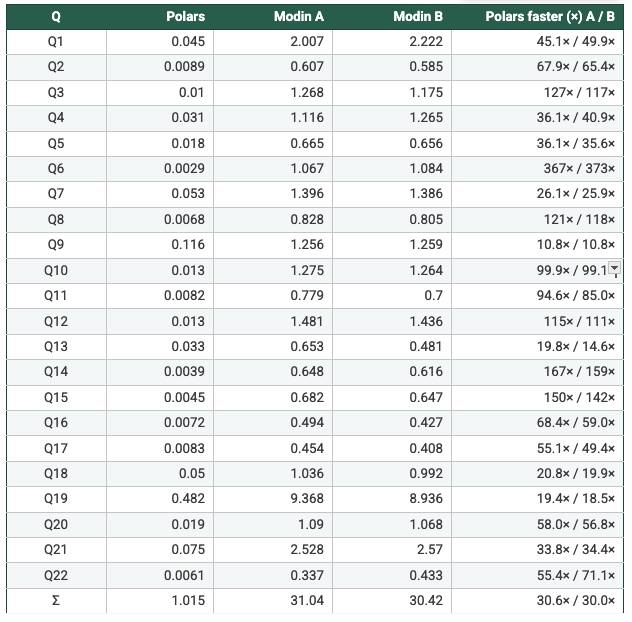
Note: the values in the tables below are in seconds.
This layout makes it explicit whether gains come from (a) the engine’s per-core efficiency, (b) scaling out across workers/cores, or (c) multi-threaded numeric kernels.
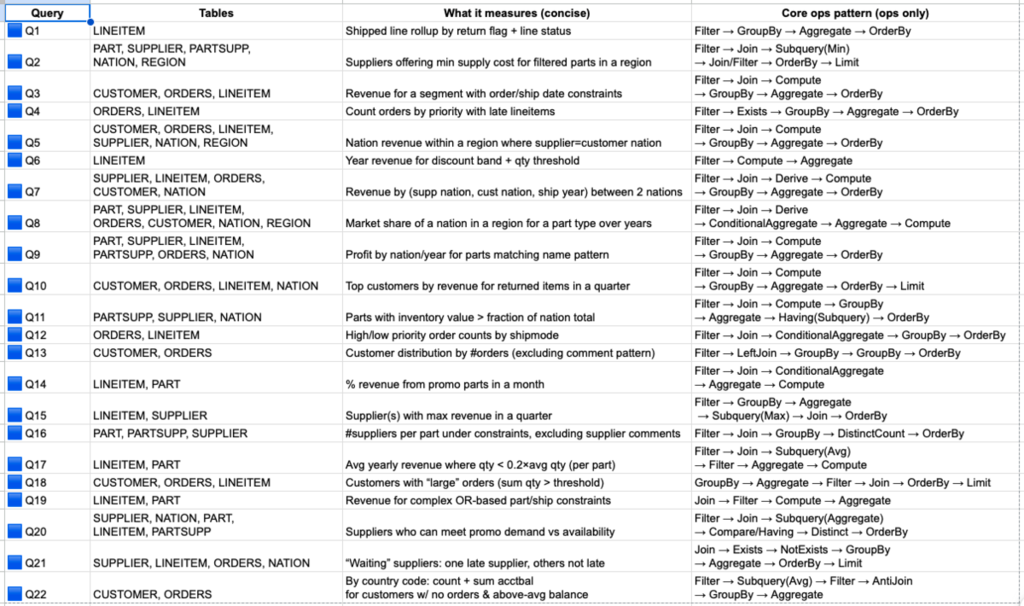
Dataset: SF=1
Report the SF=1 results for each workload under the aligned configurations below:
N = 1
- Polars: POLARS_MAX_THREADS=1
- Modin A: MODIN_CPUS=1, kernel threads=1
- Modin B: MODIN_CPUS=1, kernel threads=1
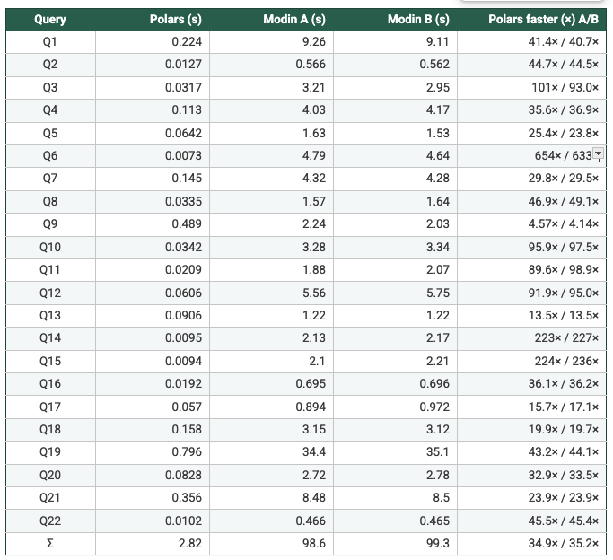
N = 2
- Polars: POLARS_MAX_THREADS=2
- Modin A: MODIN_CPUS=2, kernel threads=1
- Modin B: MODIN_CPUS=1, kernel threads=2
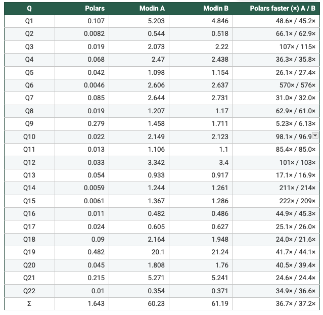
N = 4
- Polars: POLARS_MAX_THREADS=4
- Modin A: MODIN_CPUS=4, kernel threads=1
- Modin B: MODIN_CPUS=1, kernel threads=4
N = 8
- Polars: POLARS_MAX_THREADS=8
- Modin A: MODIN_CPUS=8, kernel threads=1
- Modin B: MODIN_CPUS=1, kernel threads=8
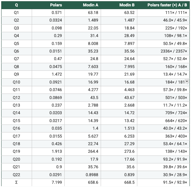
Dataset: SF=5
Repeat the same reporting structure for SF=5:
N = 1
- Polars: POLARS_MAX_THREADS=1
- Modin A: MODIN_CPUS=1, kernel threads=1
- Modin B: MODIN_CPUS=1, kernel threads=1
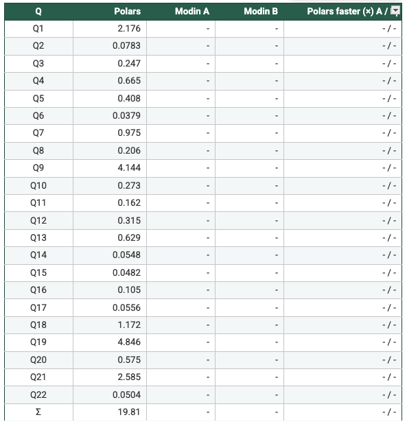
Note: The Ray engine crashed at ~minute 30 for both Modin A & Modin B, so there are no results for the two setups
N = 2
- Polars: POLARS_MAX_THREADS=2
- Modin A: MODIN_CPUS=2, kernel threads=1
- Modin B: MODIN_CPUS=1, kernel threads=2
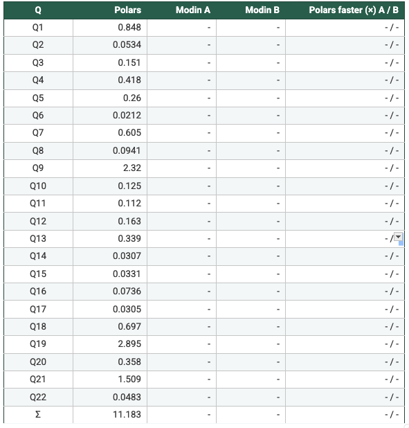
Note: I cancelled the runs for Modin A & Modin B at ~60 minutes, so there are no results for the two setups
N = 4
- Polars: POLARS_MAX_THREADS=4
- Modin A: MODIN_CPUS=4, kernel threads=1
- Modin B: MODIN_CPUS=1, kernel threads=4
N = 8
- Polars: POLARS_MAX_THREADS=8
- Modin A: MODIN_CPUS=8, kernel threads=1
- Modin B: MODIN_CPUS=1, kernel threads=8
Key Takeaways
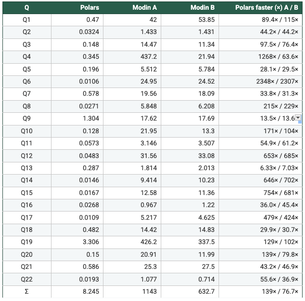
- Measured from the recorded per-query runtimes: On SF1 (N=1/2/4/8), Polars is faster than Modin Setup A and Setup B on 22/22 queries in every configuration, with geometric-mean speedups ranging from 47× to 62×. On SF5, Modin produced results only at N=4 and N=8; in those cases Polars is again faster on 22/22 queries, with geometric-mean speedups of 108×–113× vs Modin A and 93×–109× vs Modin B. Total suite time shows the same pattern (e.g., SF5 N=4: 7.199s Polars vs 658.6s Modin A vs 668.5s Modin B). So, it's clear to say Polars is consistently faster in this benchmark. Across the workloads and scale factors I ran, Polars outperformed Modin by a clear margin, suggesting the difference is structural (execution model and engine design) rather than an outlier tied to a single query.
- On a single machine, Modin’s overhead dominates. In both Modin modes I tested—(a) one worker with more intra-process threading and (b) multiple Ray workers with single-threaded kernels—execution still flows through Ray’s task scheduling and object store. For these TPC-H–style analytics on one node, the end-to-end runtime appears more sensitive to orchestration, scheduling, and garbage-collection overhead than to raw compute throughput.
- This setup favors a single-process analytic engine. The benchmark is explicitly single-node and memory-resident. In that regime, Polars’ columnar, multi-threaded engine maps naturally to the hardware, while Modin’s primary advantages (cluster-scale parallelism and distributed memory) are not exercised.
Limitations
- Single-node, in-memory focus. The results reflect a laptop-scale, single-machine scenario with RAM-resident analytics. They should not be extrapolated to multi-node clusters or workloads that exceed local memory—where Modin’s distributed design is intended to shine.
- Polars benefits from a native columnar execution engine and (optionally) lazy query planning, while Modin executes a pandas-compatible API on top of Ray. The benchmark therefore measures end-to-end systems (including orchestration and execution strategy), not only “parallelism knobs.”
- I/O is intentionally de-emphasized. Data is standardized as typed Parquet to reduce parsing/type inference costs. This makes the benchmark more representative of execution-heavy analytics, but it may understate scenarios where CSV/text ingestion is the dominant cost.